Predicting Taxi Trip Distance:

Zoning, Census, and Geographic Data Boosts Model Performance

Anna E. Jurgensen

December 4, 2017

Given the 2013 NYC taxi trip and fare data provided for the UW PCE Data Science 450 course, a model was built to predict taxi trip distance. This aim was chosen as being able to predict trip distance could potentially help a company validate reported taxi trip distances and the fares calculated from them. The following is a brief summary of my project, covering the data used, the features engineered, and the models developed. For a more detailed summary of the project, please see the pdf version of my final report.

Data Used

The taxi trip and fare data used for modeling was limited to fields of information that a driver could know at the beginning of the trip, and so excluded trip time and payment information such as fare, tip, etc. Further, using the geographic coordinates for the rides' pick-up and drop-off locations several map overlays were used to create additional features. The map overlays used were:

US Census Bureau map for determining state and county
NYC metro area zoning maps
NYC metro Neighborhood Tabulation Areas (NTAs)
locations of major NYC metro transportation hubs (airports, subway & train stations, ferry landings)

The features created from the the US Census Bureau state and county information as well as those from the NYC Neighborhood Tabulation Areas were also used to create features from American Community Survey data.

Feature Engineering

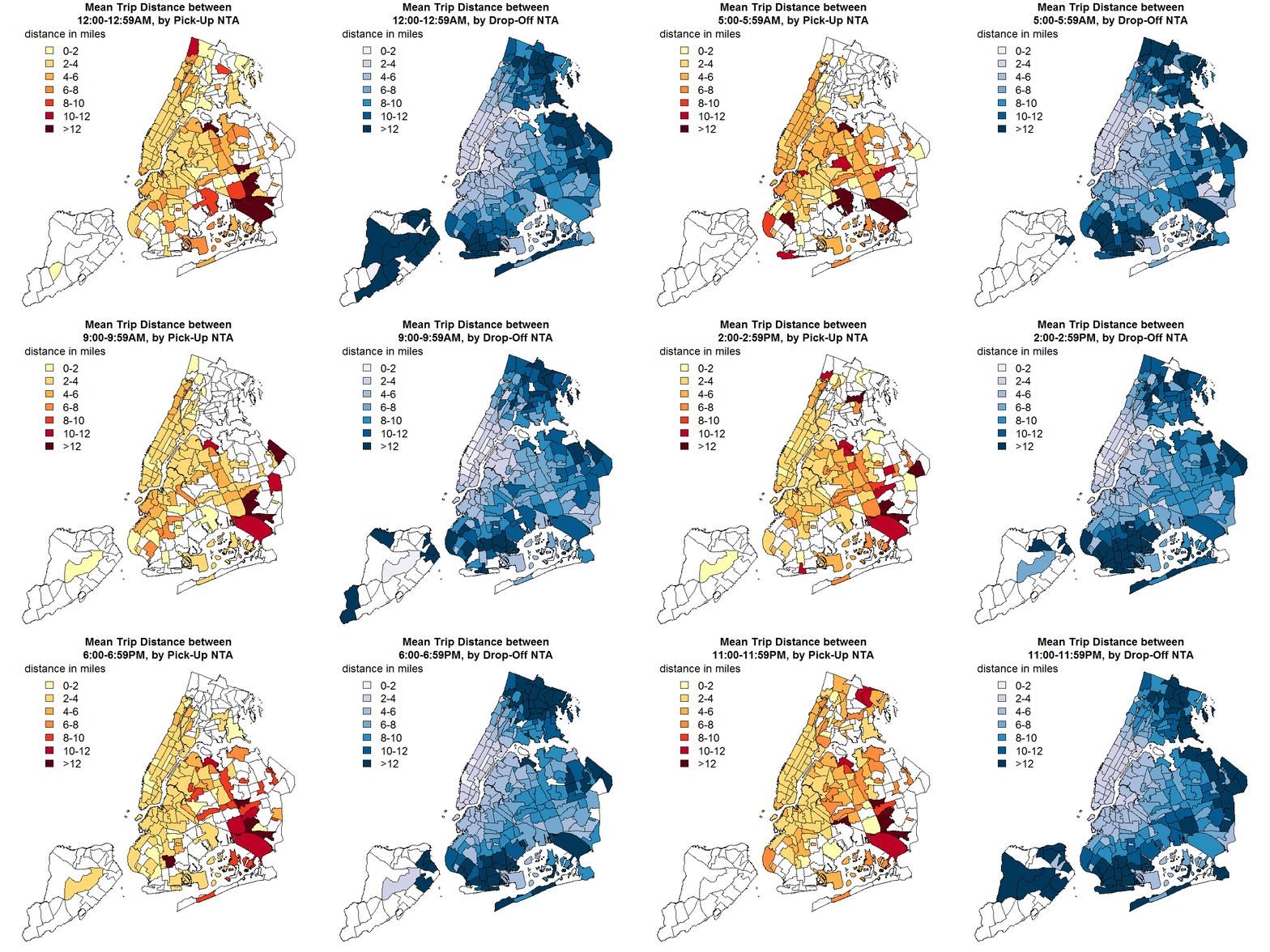
After overlaying the county and NTA maps, I noticed that average trip distances tended to be shorter or longer depending on the NTA of the trip's pick-up and drop-off.

However, simply creating basic "pick-up/drop-off in NTA/county <X>" features would be problematic for several reasons. First of all, doing so would create a very large number of features, many of which didn't have much (or any) data in the training set. Second, Creating features for each of the individual NTAs or counties would miss any meaningful similarities between these areas. Creating a small number of features based on common attributes of the geographic areas of ride pick-ups and drop-offs, then, would reduce the dimensionality of the data (thus reducing computation time and expense), and could potentially improve the predictive power of whatever ML algorithm was ultimately used.

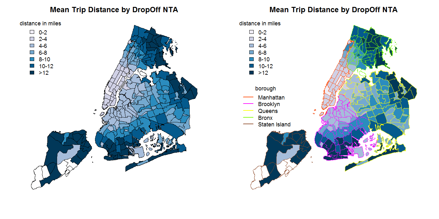
Unsurprisingly, the divisions between similar areas weren't as simple as beloning to different boroughs. For example, the gif to the right shows the unambiguous lack of alignment between drop-off NTAs with similar mean trip distances (indicated by the area's fill color) and membership in different boroughs (outline color).

To effectivtly 'describe' the environment of the pick-up and drop-off locations and to capture underlying similarities between the geographic areas, I used the NTA (for locations within the NYC metro area) or the state and county FIPs codes (for the remaining locations) to join American Community Survey data from the year prior to that of the taxi trip data (ACS 2012). From the welath of ACS data available I used only data that I thought was most likely to correlate (positively or negatively) with taxi use. In particular, for each area I retrieved:

total number of housing units
number of occupied housing units
percentage of housing units with access to 0, 1, 2, or 3 or more vehicles
total number of workers living in the area
percentage of residents that take taxis to work
percentage of workers in industries I thought were most likely to use cabs (for commuting, meetings, or travel):
- finance, real estate, and insurance
- professions, science, and management
- information

ML Model Performance

The problem of predicting a numerical distance called for a regression model. As such, I tried linear regression as well as bagging, boosted trees, and random forest training algorithms, tuning the hyperparameters of each, to find the model with the best predictive performance. Ultimately, the random forest model (converged at 48 trees with a maximum tree depth of 20) proved to have the best performance based on MAE, RMSE, and R2 (0.372, .0785, 0.933, respectively).

Lastly, to test whether the model performed better than a mere "best guess" of what any random taxi ride's distance would be, I created two benchmark models by taking as the predicted distance for all observations of the testing set either the mean or the median trip distance from the training set. Additionally, to test whether the features I had created from outside data had actually improved the model, I compared performance of the final 149 features in a random forest model with 20 trees and a max tree depth of 20 to models with the same hyperparameters using (a) just features from the original taxi data or (b) just features created from outside data sources. The performance metrics for these five models are listed in the table below. Comparing these metrics, it is clear that any of the models using developed features perform much better than the "best guess" benchmark models (compare R2 values of 0.898 and above for the models from developed features to 0.000 and 0.108 for the "best guess" benchmark models). Further, from comparing the performance of the final model to the model using only features from the original taxi data, we can see from the lower error rates (MAE and RMSE) and higher coefficient of determination (R2) that the features created from outside data did in fact improve model performance. Lastly, and surprisingly, it appears that the features from outside data not only improved the taxi data-only model, they also perform quite well on their own, with MAE and RMSE rates only a bit higher than those for the taxi data-only model, and an R2 rate only a bit lower. Ultimately my conclusion is that the feature creation from oustide data sources was successful.

Model	MAE	RMSE	R2
mean distance (2.805 mi) as predicted distance	1.948	3.044	0.000
median distance (1.800 mi) as predicted distance	1.714	3.204	0.108
just features from original taxi data	0.563	0.909	0.911
just features from outside data sources	0.549	0.974	0.898
final feature set at 20 trees	0.377	0.792	0.932
final feature set (converged at 48 trees)	0.372	0.785	0.933